DenseNet - Densely Connected Convolutional Networks

DenseNets have several important contributions to the field of computer vision, including:

1. Addressing the vanishing gradient problem: DenseNets connect each layer to every other layer in a feedforward manner, allowing for a direct flow of gradients throughout the network. This helps to alleviate the vanishing gradient problem and enables the efficient training of very deep networks.
2. Reducing the number of parameters: By connecting each layer to every other layer, DenseNets can reuse feature maps from earlier layers, reducing the number of parameters needed in the network. This makes them more memory-efficient and easier to train than traditional convolutional neural networks (CNNs).
3. Improving feature propagation: The dense connectivity in DenseNets allows for more direct information flow between layers, which leads to improved feature propagation and feature reuse. This, in turn, results in better model accuracy, especially for smaller datasets.

Main Ideas

For each layer, the feature maps of all preceding layers are used as inputs, and its own feature-maps are used as inputs into all subsequent layers.

Authors alleviate the vanishing-gradient problem, strengthen feature propagation, encourage feature reuse, and substantially reduce the number of parameters.

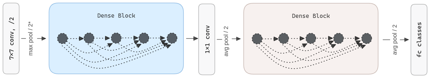
To ensure maximum information flow between layers in the network, all layers are connected (with matching feature-map sizes) directly with each other. To preserve the feed-forward nature, each layer obtains additional inputs from all preceding layers and passes on its own feature maps to all subsequent layers. Authors combine features by concatenating them.

Dense connectivity. To further improve the information flow between layers, we propose a different connectivity pattern: we introduce direct connections from any layer to all subsequent layers. Consequently, the $l^{th}$ layer receives the feature maps of all preceding layers, $x_0, \dots, x_{l-1}$, as input: $x_l = H_l([x_o, x_1, \dots, x_{l-1}])$ where $[x_o, x_1, \dots, x_{l-1}]$ refers to the concatenation of the feature maps produced in layers $0, \dots, l-1$.

Pooling layers. The concatenation operation is not viable when the size of feature maps changes. However, an essential part of convolutional networks is down-sampling layers that change the size of feature maps. To facilitate down-sampling in the architecture, we divide the network into multiple densely connected dense blocks. We refer to layers between blocks as transition layers, which do convolution and pooling. The transition layers used in the experiments consist of a batch normalization layer and a 1×1 convolutional layer followed by a 2×2 average pooling layer.

Growth rate. If each function $H_l$ produces k feature maps, it follows that the $l^{th}$ layer has $k_o + k \times(l-1)$ input feature maps, where $k_0$ is the number of channels in the input layer. An important difference between DenseNet and existing network architectures is that DenseNet can have very narrow layers, e.g., k = 12. We refer to the hyperparameter k as the growth rate of the network.

Bottleneck layers. Although each layer only produces k output feature maps, it typically has many more inputs. A 1×1 convolution can be introduced as a bottleneck layer before each 3×3 convolution to reduce the number of input feature maps and thus improve computational efficiency. We find this design especially effective for DenseNet

Architecture & Training Details

Authors use 1×1 convolution followed by 2×2 average pooling as transition layers between contiguous dense blocks. At the end of the last dense block, a global average pooling is performed. SGD with 0.1 learning rate and batch size 256 is used.

DenseNet architectures for ImageNet. The growth rate for all the networks is k = 32. Note that each “conv” layer shown in the table corresponds the sequence BN-ReLU-Conv.

Output size	121-layer	169-layer	201-layer	264-layer
112x112	7x7, 64, stride 2, pad 3
56x56	3x3 max pool, stride 2
	$\begin{bmatrix}1 \times 1 \, \textnormal{conv}\\ 3 \times 3 \, \textnormal{conv}\end{bmatrix}\times 6$	$\begin{bmatrix}1 \times 1 \, \textnormal{conv}\\ 3 \times 3 \, \textnormal{conv}\end{bmatrix}\times 6$	$\begin{bmatrix}1 \times 1 \, \textnormal{conv}\\ 3 \times 3 \, \textnormal{conv}\end{bmatrix}\times 6$	$\begin{bmatrix}1 \times 1 \, \textnormal{conv}\\ 3 \times 3 \, \textnormal{conv}\end{bmatrix}\times 6$
28x28	1x1 conv + 2x2 avg pool, stride 2
	$\begin{bmatrix}1 \times 1 \, \textnormal{conv}\\ 3 \times 3 \, \textnormal{conv}\end{bmatrix}\times 12$	$\begin{bmatrix}1 \times 1 \, \textnormal{conv}\\ 3 \times 3 \, \textnormal{conv}\end{bmatrix}\times 12$	$\begin{bmatrix}1 \times 1 \, \textnormal{conv}\\ 3 \times 3 \, \textnormal{conv}\end{bmatrix}\times 12$	$\begin{bmatrix}1 \times 1 \, \textnormal{conv}\\ 3 \times 3 \, \textnormal{conv}\end{bmatrix}\times 12$
14x14	1x1 conv + 2x2 avg pool, stride 2
	$\begin{bmatrix}1 \times 1 \, \textnormal{conv}\\ 3 \times 3 \, \textnormal{conv}\end{bmatrix}\times 24$	$\begin{bmatrix}1 \times 1 \, \textnormal{conv}\\ 3 \times 3 \, \textnormal{conv}\end{bmatrix}\times 32$	$\begin{bmatrix}1 \times 1 \, \textnormal{conv}\\ 3 \times 3 \, \textnormal{conv}\end{bmatrix}\times 48$	$\begin{bmatrix}1 \times 1 \, \textnormal{conv}\\ 3 \times 3 \, \textnormal{conv}\end{bmatrix}\times 64$
7x7	1x1 conv + 2x2 avg pool, stride 2
	$\begin{bmatrix}1 \times 1 \, \textnormal{conv}\\ 3 \times 3 \, \textnormal{conv}\end{bmatrix}\times 16$	$\begin{bmatrix}1 \times 1 \, \textnormal{conv}\\ 3 \times 3 \, \textnormal{conv}\end{bmatrix}\times 32$	$\begin{bmatrix}1 \times 1 \, \textnormal{conv}\\ 3 \times 3 \, \textnormal{conv}\end{bmatrix}\times 32$	$\begin{bmatrix}1 \times 1 \, \textnormal{conv}\\ 3 \times 3 \, \textnormal{conv}\end{bmatrix}\times 48$
1x1	average pool + fully connected [classes] + softmax

Code

The DenseLayer receives the concatenated feature maps from all previous layers and produces k new feature-maps using a 3×3 convolution. Note that previously, the number of feature-maps is reducede by a 1×1 convolution.

class DenseLayer(nn.Module):
    def __init__(self, num_input_features, growth_rate, bn_size):
        super(DenseLayer, self).__init__()
        self.norm1 = nn.BatchNorm2d(num_input_features)
        self.relu1 =  nn.ReLU(inplace=True)
        self.conv1 = nn.Conv2d(
            num_input_features, bn_size * growth_rate,
            kernel_size=1, stride=1, bias=False
        )
        
        self.norm2 = nn.BatchNorm2d(bn_size * growth_rate)
        self.relu2 = nn.ReLU(inplace=True)
        self.conv2 = nn.Conv2d(
            bn_size * growth_rate, growth_rate,
            kernel_size=3, stride=1, padding=1, bias=False
        )

    def forward(self, concated_features):
        bottleneck_output = self.conv1(self.relu1(self.norm1(concated_features)))
        new_features = self.conv2(self.relu2(self.norm2(bottleneck_output)))
        
        return new_features

If we take this DenseLayer and stack it several times, we get a DenseBlock. We can see how the features that every DenseLayer produce are concatenatedover the features list and passed to the next DenseLayer. Also, the number of input features is increased by the growth rate at each iteration.

class DenseBlock(nn.ModuleDict):
    def __init__(self, num_layers, num_input_features, bn_size, growth_rate):
        super(DenseBlock, self).__init__()
        self.dense_layers = []
        for i in range(num_layers):
            layer = DenseLayer(
                num_input_features + i * growth_rate,
                growth_rate=growth_rate,
                bn_size=bn_size
            )
            self.dense_layers.append(layer)

    def forward(self, init_features):
        features = [init_features]
        for layer in self.dense_layers:
            concated_features = torch.cat(features, 1)
            new_features = layer(concated_features)
            features.append(new_features)
            
        return torch.cat(features, 1)

The last building block is the transition layer, which is composed of a batch normalization layer and a 1×1 convolutional layer followed by a 2×2 average pooling layer.

class Transition(nn.Sequential):
    def __init__(self, num_input_features, num_output_features):
        super(Transition, self).__init__()
        self.norm = nn.BatchNorm2d(num_input_features)
        self.relu = nn.ReLU(inplace=True)
        self.conv = nn.Conv2d(
            num_input_features, num_output_features,
            kernel_size=1, stride=1, bias=False
        )
        self.pool = nn.AvgPool2d(kernel_size=2, stride=2)

    def forward(self, x):
        out = self.conv(self.relu(self.norm(x)))
        out = self.pool(out)
        
        return out

With these three building blocks, we can define the DenseNet architecture.

class DenseNet(nn.Module):
    """
    Args:
        growth_rate (int) - how many filters to add each layer (`k` in paper)
        block_config (list of 4 ints) - how many layers in each pooling block
        num_init_features (int) - the number of filters to learn in the first convolution layer
        bn_size (int) - multiplicative factor for number of bottle neck layers
          (i.e. bn_size * k features in the bottleneck layer)
        num_classes (int) - number of classification classes
    """

    def __init__(self, growth_rate=32, block_config=(6, 12, 24, 16),
                 num_init_features=64, bn_size=4, num_classes=1000):

        super(DenseNet, self).__init__()
        
        # First convolution
        self.features = nn.Sequential(
            nn.Conv2d(
                3, num_init_features,
                kernel_size=7, stride=2, padding=3, bias=False
            ),
            nn.BatchNorm2d(num_init_features),
            nn.ReLU(inplace=True),
            nn.MaxPool2d(kernel_size=3, stride=2, padding=1),
        )

        # Each denseblock
        num_features = num_init_features
        for i, num_layers in enumerate(block_config):
            block = DenseBlock(
                num_layers=num_layers,
                num_input_features=num_features,
                bn_size=bn_size,
                growth_rate=growth_rate
            )
            self.features.append(block)
            
            num_features = num_features + num_layers * growth_rate
            
            if i != len(block_config) - 1:
                trans = Transition(
                    num_input_features=num_features,
                    num_output_features=num_features // 2
                )
                self.features.append(trans)
                num_features = num_features // 2

        # Final batch norm
        self.features.append(nn.BatchNorm2d(num_features))

        # Linear layer
        self.classifier = nn.Linear(num_features, num_classes)

    def forward(self, x):
        features = self.features(x)
        out = F.relu(features, inplace=True)
        out = F.adaptive_avg_pool2d(out, (1, 1))
        out = torch.flatten(out, 1)
        out = self.classifier(out)
        return out

And that’s it! We can now instantiate, for example, a DenseNet-121.

densenet121 = DenseNet(32, (6, 12, 24, 16), 64)

Credits

• Paper - Densely Connected Convolutional Networks