
Transformer architecture is everywhere today. The core idea, even with differences, adjustments and tweaks remains state of the art in multiple tasks, from natural language processing to computer vision. In the following post I will try to give a simple but complete approach to how the Transformer works, so that we can understand future derivatives of this architecture.
We will divide the explanation by the different parts that compose the model. I may omit some super technical or mathematical details in order to digest this better, so I recommend you refer to the original paper that you can find at the end of the post. Let’s go, from the beginning, block by block.
Overview
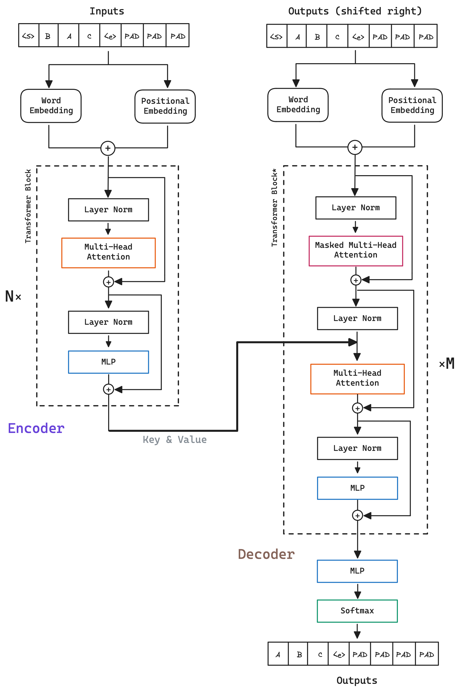
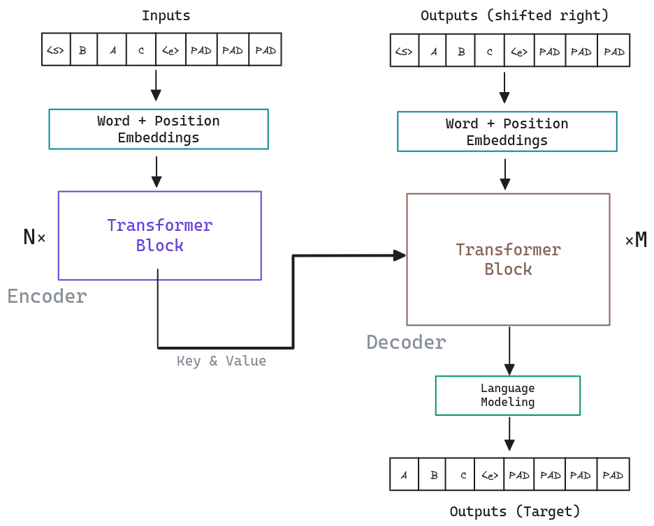
The Transformer is a model that works with sequences of data. It is composed of two parts, the encoder and the decoder.
The Encoder is in charge of transforming the input into a representation that the decoder can understand. The Decoder is in charge of generating the output based on the representation that the encoder has generated.
Although different variants of the model have been proposed and encoder only and decoder only models have been used, we will focus on the original model, which is composed of both parts. Let’s see a visual representation of the model.
Transforming the input
Throughout the post we will use a natural language example to explain the model. To be able to use the words, we need to transform them into something that the model can understand, into numbers. The easiest way to do this is to use a dictionary, where each word has a unique number associated. This dictionary is also known as Vocabulary.
Imagine that we want to tackle a problem where we want to sort a list of characters. The set of characters that we can use is “A”, “B”, and “C”. Our vocabulary could be:
vocabulary = {
    "PAD": 0,
    "<s>": 1,
    "<e>": 2,
    "A": 3,
    "B": 4,
    "C": 5
}
Note that we have added three special tokens, PAD, <s> and <e>. These are common
tokens used for different purposes:
PAD: Padding token. It is used to fill the input to the same length. We need to do this because to be able to process the input in batches, all the inputs must have the same length, so shorter inputs are filled with this token till they reach the maximum length.<s>: Start token. It is used to indicate the beginning of the input.<e>: End token. It is used to indicate the end of the input.
These representations of word mappings are known as Tokens.
Once we have converted the words to something the model can understand it is time to give them power. To do this, we are going to transform the flat, simple representations of our vocabulary into something richer and that captures the semantic relationships, the meaning of the word, and how it relates to other words. But, how can we do that? Is something that the model needs to learn through what is known as embeddings. The embeddings are just a learnable representation that we help us to continue transforming the input into something that the model can work with. Will work as a lookup table, where each word is represented by a vector of numbers. This embeddings are known as Word Embeddings.
Finally, in addition to capturing the essence of the words, it is important to capture the position of the words. The model by itself does not know the order of the words, so we need to add this information. Although the original paper uses a different approach, we will use a simpler and more widely used approach, which is to add learned embeddings for each position in the input. This vectors are known as Positional Embeddings and work in a similar lookup table way as the word embeddings, but instead of representing the meaning of the word, they represent the position of the word in the input.
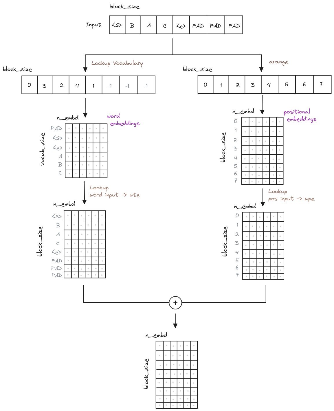
So, we have the word embeddings and the positional embeddings, but how do we combine them? Well, we just add them together. This is the input that we will give to the model.
Here is a visual representation of the input transformation. The block_size is the maximum
length of the input, the vocab_size is the size of the vocabulary, and the n_embd is the
size of the learned embeddings.
We can start our code defining the embeddings and how to combine them. This part is the same for the Encoder and the Decoder.
class Encoder(nn.Module):  # either Encoder or Decoder

    def __init__(self, config):
        super().__init__()
        self.wte = nn.Embedding(config.vocab_size, config.n_embd)
        self.wpe = nn.Embedding(config.block_size, config.n_embd)
        self.drop = nn.Dropout(config.dropout)
        # ...

     def forward(self, x, targets=None):
        b, t = x.size()  # batch size, block_size
        # generate the position indices for the lookup positional embeddings table
        pos = torch.arange(0, t) # shape (block_size)

        # forward the Word Embeddings, Positional Embeddings and add them together
        tok_emb = self.wte(x) # token embeddings of shape (batch, block_size, n_embd)
        pos_emb = self.wpe(pos) # position embeddings of shape (block_size, n_embd)
        x = self.drop(tok_emb + pos_emb)  # shape (batch, block_size, n_embd)
        # ...
The Transformer Block
We have transformed the input into something that the model can understand, but how does the model work? The model is composed of a block that is repeated multiple times. This block mission is to understand the relations of input and output sequences through the training process. This block is known as Transformer Block.
The Transformer Block is composed of different parts, let’s see them one by one.
Layer Normalization
Normalization is always good, isn’t it? Well, in this case it is. The Layer Normalization is a technique that helps the model to converge faster and to generalize better. Normalizing across all features but for each of the inputs to a specific layer removes the dependence on batches. This makes layer normalization well suited for sequence models such as the Transformer, because the model is trained with sequences of different lengths.
Multi-Head Attention
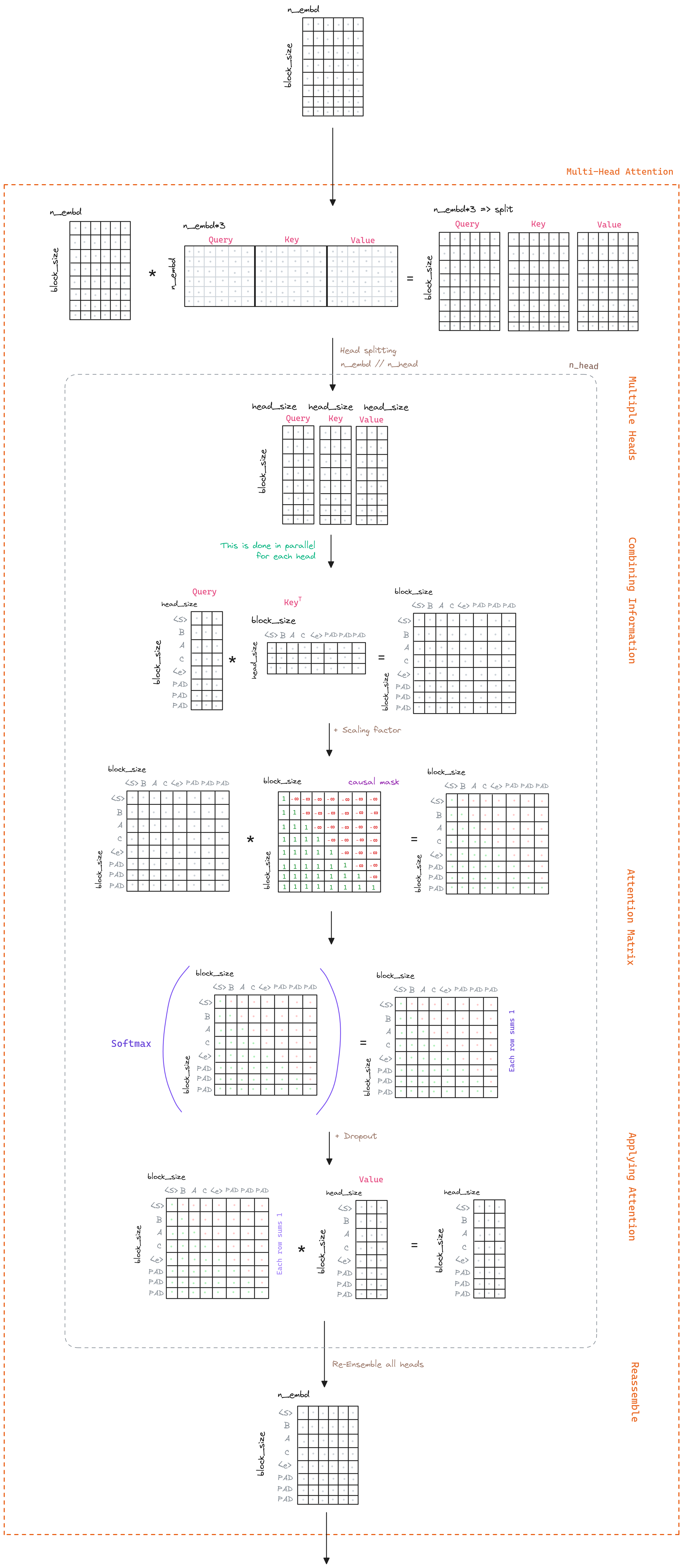
The core of the Transformer is the Multi-Head Attention. This part is responsible for capturing the relationships between the tokens in the sequence. It is composed of three parts, the query, the key and the value. Those parts are combined to generate the attention matrix, which is used to capture the relationships between the tokens.
Although at the end of the day what happens behind the neural networks is a bit of magic, the intuition is as follows:
The key/value/query concept is analogous to retrieval systems. For example, when you search for videos on Youtube, the search engine will map your query (text in the search bar) against a set of keys (video title, description, etc.) associated with candidate videos in their database, then present you the best matched videos (values).
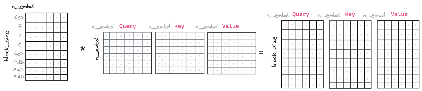
So the process starts by generating the query, key and value vectors given the input sequence we transformed earlier (Transforming the input). We do that by applying a linear transformation, a matrix multiplication, to the input.
class MultiHeadAttention(nn.Module):
def __init__(self, config):
super(MultiHeadAttention, self).__init__()
self.config = config
# key, query and value matrixes
self.query_matrix = nn.Linear(
config.n_embd, config.n_embd, bias=config.bias
)
self.key_matrix = nn.Linear(
config.n_embd, config.n_embd, bias=config.bias
)
self.value_matrix = nn.Linear(
config.n_embd, config.n_embd, bias=config.bias
)
# ...
def forward(self, key, query, value, mask=None):
query = self.query_matrix(query)
key = self.key_matrix(key)
value = self.value_matrix(value)
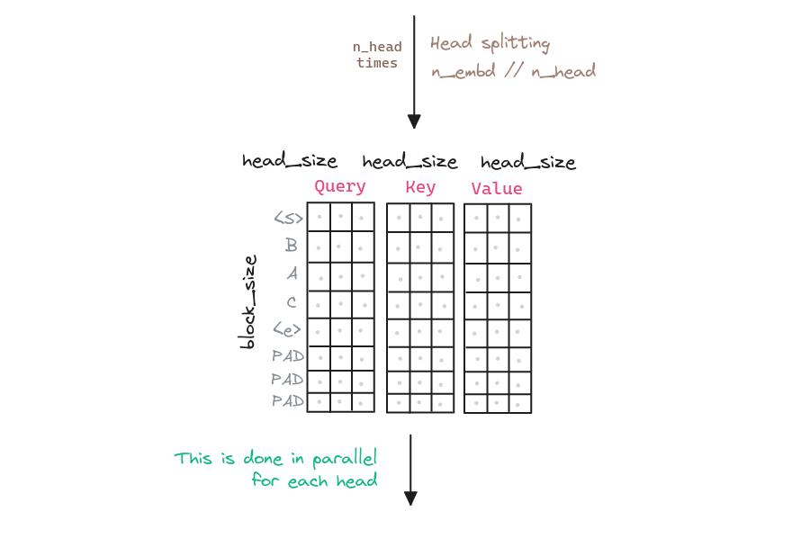
# ...Next the multi-head part comes into play. The idea is to generate multiple query, key and value vectors, and then combine them. This is done to capture different relationships between the tokens: syntactic, semantic, spatial, etc. The number of heads is a hyperparameter of the model. For more information about the intuition behind the multiple heads, refer to the FAQ section.
class MultiHeadAttention(nn.Module):
    def __init__(self, config):
        super(MultiHeadAttention, self).__init__()
        # ...

    def forward(self, key, query, value, mask=None):
        # ...
        batch_size, block_size = key.size(0), key.size(1)
        # each key, query, value will be of n_embd / n_heads
        single_head_size = self.config.n_embd // self.config.n_heads
        # query size can change in decoder during inference,
        block_size_query = query.size(1)

        # (batch, block_size, n_embd) -> (batch, block_size, n_heads, n_embd / n_heads)
        # transpose to (batch, n_heads, block_size, n_embd / n_heads)
        query = query.view(
            batch_size, block_size_query, self.config.n_heads, single_head_size
        ).transpose(1, 2)
        key = key.view(
            batch_size, block_size, self.config.n_heads, single_head_size
        ).transpose(1, 2)
        value = value.view(
            batch_size, block_size, self.config.n_heads, single_head_size
        ).transpose(1, 2)
        # ...
With each of the query, key and value vectors generated, we can now generate the attention matrix. This matrix is generated by applying the dot product between the query and the key vectors. The purpose of this is to capture the relationships between the tokens. The higher the dot product, the higher the relationship between the tokens. The dot product is then scaled by the square root of the dimension of the key vectors. This is done to avoid the dot product to be too large, which would make the softmax function to saturate.
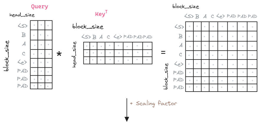
class MultiHeadAttention(nn.Module):
    def __init__(self, config):
        super(MultiHeadAttention, self).__init__()
        # ...

    def forward(self, key, query, value, mask=None):
        # ...
        # Compute the attention matrix
        att = query @ key.transpose(-2, -1)
        # Scale the attention matrix
        att = att  / math.sqrt(single_head_size)
        # ...
Once we have the attention matrix, we can apply the softmax function to it. This will generate a matrix where each row will sum to 1. This matrix is known as the attention weights. On top of this matrix we can apply a Dropout layer to avoid overfitting.
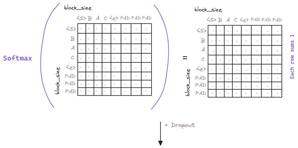
class MultiHeadAttention(nn.Module):
    def __init__(self, config):
        super(MultiHeadAttention, self).__init__()
        # ...
        self.attn_dropout = nn.Dropout(config.dropout)

    def forward(self, key, query, value, mask=None):
        # ...
        # Apply the softmax function to the attention matrix
        att = F.softmax(att, dim=-1)
        att = self.attn_dropout(att)
        # ...
And now we can apply the attention weights to the value vectors. This will generate the context vectors. This vectors are the ones that will be used by the model to condition the decoder and generate the output, as the encoder and the decoder use similar attention mechanisms.
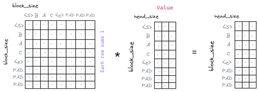
class MultiHeadAttention(nn.Module):
    def __init__(self, config):
        super(MultiHeadAttention, self).__init__()
        # ...

    def forward(self, key, query, value, mask=None):
        # ...
        # Multiply the attention weights by the value vectors
        out = att @ value
        # ...
Rembember that we have multiple heads, so we need to combine them. This is done by concatenating the context vectors.
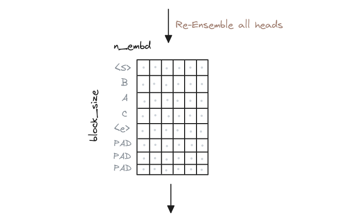
class MultiHeadAttention(nn.Module):
    def __init__(self, config):
        super(MultiHeadAttention, self).__init__()
        # ...

    def forward(self, key, query, value, mask=None):
        # ...
        # Re-assemble all head outputs side by side
        # From (batch, n_heads, block_size, n_embd / n_heads)
        # -> to (batch, block_size, n_heads, n_embd / n_heads)
        out = out.transpose(1, 2).contiguous().view(
            batch_size, block_size_query, self.config.n_embd
        )
        return out
And that’s all for the Multi-Head Attention. The intuition is that we have generated a representation of the input that captures the relationships between the tokens.
As a quick recap, the Multi-Head Attention is composed of the following steps:
Masked Multi-Head Attention
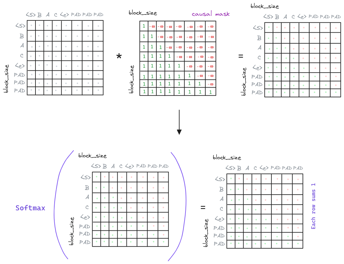
Also known as causal multi-head attention, this part is similar to the multi-head attention but with a small difference: the attention is masked. This is done because at Inference Time a given generated token can only attend to the previous generated tokens, as does not have access to the future tokens. To simulate this behavior, we mask the attention matrix at training time.
Overwriting the procedure seen in the Multi-Head Attention section, we will add an additional step masking the attention matrix before applying the softmax.
class MultiHeadAttention(nn.Module):
    def __init__(self, config):
        super(MultiHeadAttention, self).__init__()
        # ...
        # causal mask to ensure that attention
        # is only applied to the left in the input sequence
        self.mask = torch.tril(
            torch.ones(
                config.block_size, config.block_size
            )
        ).view(1, 1, config.block_size, config.block_size)

    def forward(self, key, query, value, add_mask=False):
        # ...
        # Add the mask to the attention matrix
        if add_mask:
            att = att.masked_fill(
                self.mask[:, :, :self.config.block_size, :self.config.block_size] == 0,
                float('-inf')
            )
        # Apply the softmax function to the attention matrix
        att = F.softmax(att, dim=-1)
        # ...
With this, we ensure that the model can only attend to the previous tokens as the future tokens are zeroed out.
Feed Forward - MLP
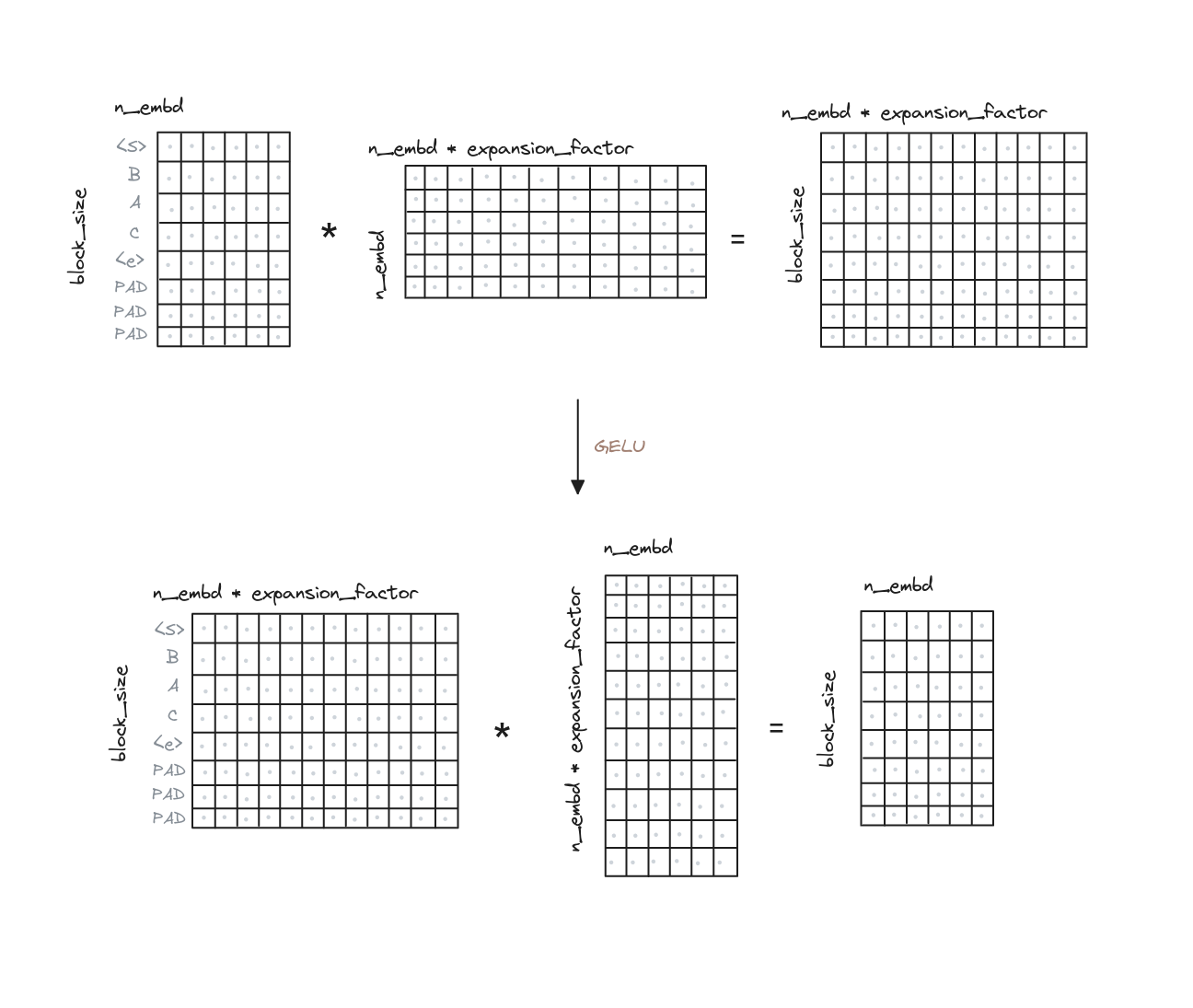
The Feed Forward layer is a simple linear transformation followed by a non-linear activation function. In this case there are two linear transformations, one that expands the dimensionality of the input by an arbitrary factor, and another that reduces it back to the original dimensionality. This combination of expanding and reducing the dimensionality of the input, adding in between a non-linear activation function, helps the model effectively capture complex patterns in the input data while maintaining computational efficiency and preventing overfitting.
class MLP(nn.Module):

    def __init__(self, config):
        super().__init__()
        self.c_fc    = nn.Linear(config.n_embd, 4 * config.n_embd, bias=config.bias)
        self.gelu    = nn.GELU()
        self.c_proj  = nn.Linear(4 * config.n_embd, config.n_embd, bias=config.bias)
        self.dropout = nn.Dropout(config.dropout)

    def forward(self, x):
        x = self.c_fc(x)
        x = self.gelu(x)
        x = self.c_proj(x)
        x = self.dropout(x)
        return x
Residual Connections
As you can observe the output of the Layer Normalization, the Multi-Head Attentions, the Masked Multi-Head Attention, and the Feed Forward layers are the same size as the input. To allow the gradients to flow better through the model, we add residual connections through the Transformer Block. Particularly after applying the Layer Normalization and some transforming layer, as the Multi-Head Attention and the Feed Forward layers. Refer to the Overview section to see the visual representation of the Transformer Block and how the residual connections are added along the Transformer Block.
As an example, we can see how the residual connections are added to the Multi-Head Attention and the Feed Forward layers in the Encoder Block.
class EncoderBlock(nn.Module):

    def __init__(self, config):
        super().__init__()
        self.ln_1 = nn.LayerNorm(config.n_embd, bias=config.bias)
        self.attn = MultiHeadAttention(config)
        self.ln_2 = nn.LayerNorm(config.n_embd, bias=config.bias)
        self.mlp = MLP(config)

    def forward(self, x):
        x = x + self.attn(self.ln_1(x))
        x = x + self.mlp(self.ln_2(x))
        return x
The Output
Once the input of the Encoder and the Decoder has been combined and transformed by the Transformer Blocks, it is time to generate the output. The output is generated by applying a linear transformation to the output of the last Decoder Transformer Block. This linear transformation is known as Language Modeling Head.
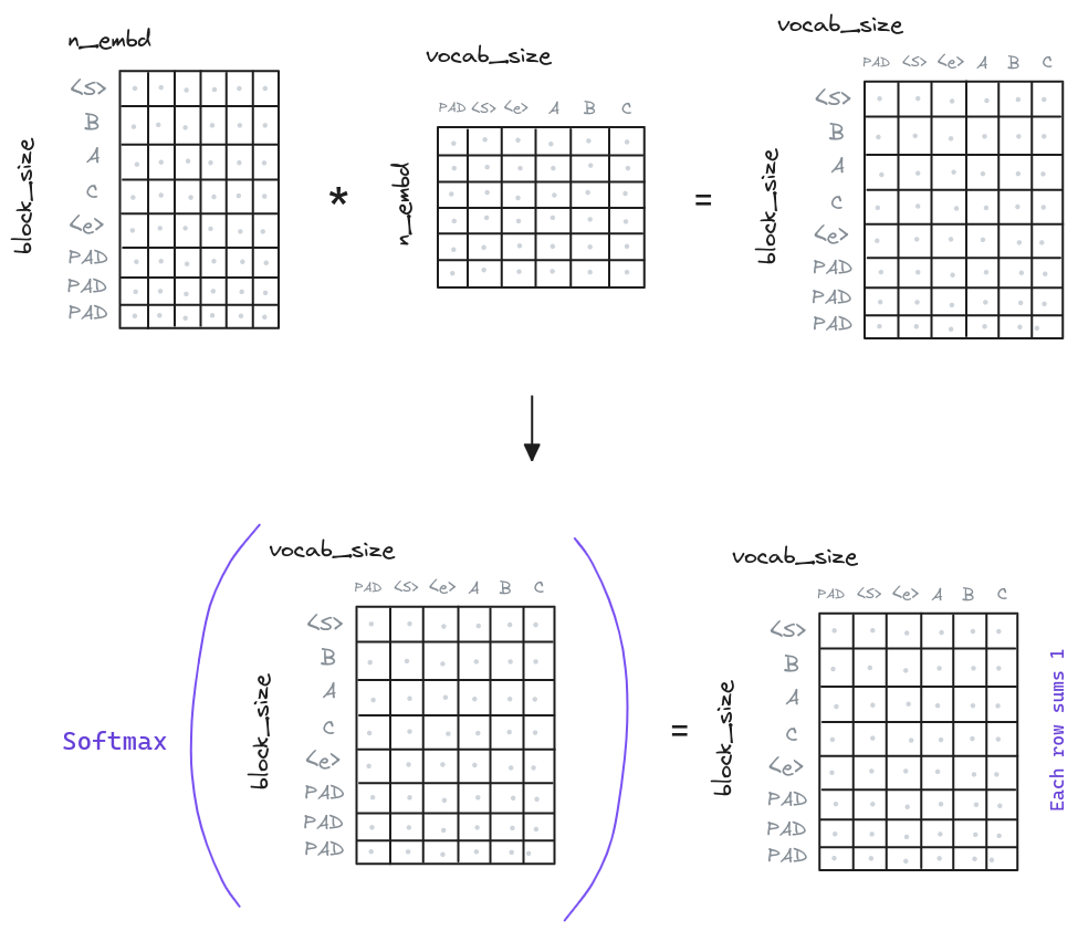
Each embedding of the sequence is multiplied by a matrix of weights that maps those embeddings to the vocabulary. That is to say, each row model the probabilities (after the softmax) of that each token (row) produces each of the tokens present in the vocabulary.
class Encoder(nn.Module):  # Decoder does not apply the LM Head

    def __init__(self, config):
        super().__init__()
        # ...
        self.lm_head = nn.Linear(config.n_embd, config.vocab_size, bias=config.bias)
        # ...

     def forward(self, x, targets=None):
        # ...
        logits = self.lm_head(x)
        # Now you can compute the loss or probabilities
        # ...
Note: For padding tokens the loss is not computed.
Last Details
We have seen the main parts of the Transformer, but there are some details that we need to take into account and can help us to have a deeper understanding of the model.
Training Time
One of the main advantages of the Transformer is that it can be trained in one step, in contrast to the recurrent neural networks that need to be trained in autoregressive fashion. This is in part thanks to the Masked Multi-Head Attention, which allows the model to attend to the previous tokens, but not to the future tokens. This allow us to use batches of data, which makes the training process faster. To do so we just need to pack token sequences of the same length in the same batch, for example by using padding (pack_padded_sequence function).
A schematic representation of the training process would be:
Inference Time
At inference time, the model is used to generate the output sequence. This is done
by generating the output token by token, also known as auto-regressive.
This is because the output of a given token depends on the previous tokens, so we need
those tokens to generate the next one. This is why we need to shift right the output,
so that the first token is the start token <s> because we don’t have any previous token.
The process would look like:
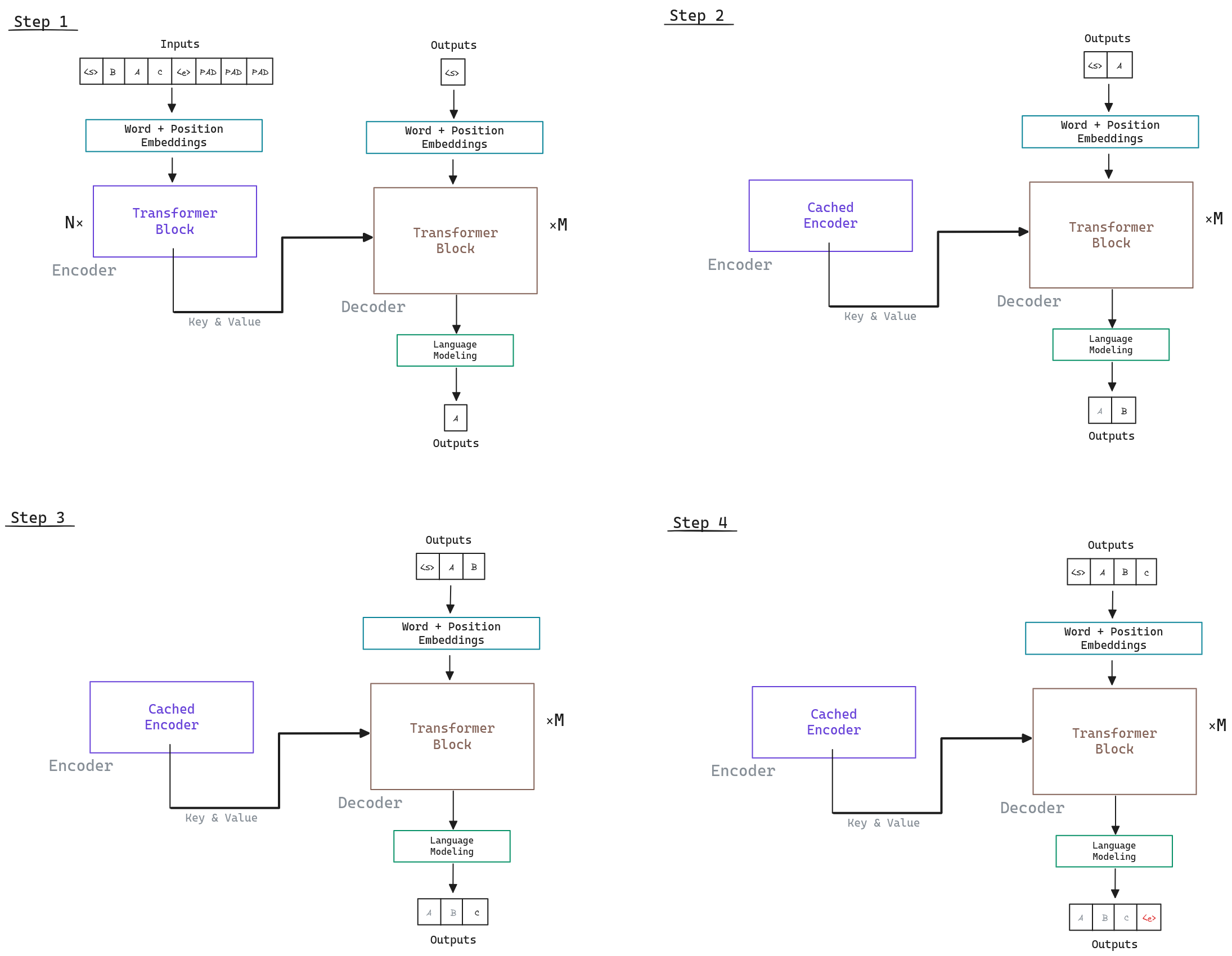
Several things to note:
- As the tokens are generated one by one, they are introduced in the input of the Decoder to generate the next token. Only the output of the last token in the Language Modeling Head is used to generate the next token, but we need to keep the rest of the tokens in the process as they are used in combination in the Multi-Head Attention.
- The Encoder output can be cached and reused for each token generated by the Decoder, as the input of the Decoder is the same for each token generated.
- The generation process can finish when the end token
<e>is generated, or when a maximum number of tokens is generated.
As an example, imagine we want to generate an arbitrary sequence of new_tokens length,
the process would look like:
encoder_out = encoder(input_sequence)
decoder_out = torch.tensor([[vocab["<s>"]]])
for _ in range(new_tokens):
    # forward the model to get the logits for the index in the sequence
    logits = decoder(encoder_out, decoder_out)
    # pluck the logits at the final step and scale by desired temperature
    # logits shape (batch, block_size, vocab_size)
    logits = logits[:, -1, :] / temperature
    # optionally crop the logits to only the top k options
    if top_k is not None:
        v, _ = torch.topk(logits, min(top_k, logits.size(-1)))
        logits[logits < v[:, [-1]]] = -float('Inf')
    # apply softmax to convert logits to (normalized) probabilities
    probs = F.softmax(logits, dim=-1)
    # sample from the distribution
    next_token = torch.multinomial(probs, num_samples=1)
    # append sampled index to the running sequence and continue
    decoder_out = torch.cat((decoder_out, next_token), dim=1)
This is a minimal example of how to generate a sequence of tokens using the Transformer. There are a lot of sampling techniques that can be used to generate the output, but that is out of the scope of this post. Note how we are using a temperature to scale the logits. This is done to control the randomness of the output. The higher the temperature, the more random the output will be.
FAQ
Why multiple heads?
The intuition is that we have generated a representation of the input that captures the relationships between the tokens. But, how do we know that the model has captured all the relationships? Well, we don’t know. But we can try to capture different relationships by generating multiple query, key and value vectors, and then combine them. This is done to capture different relationships between the tokens: syntactic, semantic, spatial, etc.
But how really works? Its all about the Query and Key multiplication. Suppose that we have just our one initial embedding representation. When we perform our Query and Key multiplication with our single embedding, we would en up with a single attention matrix. This matrix is used to capture the relationships between the tokens, empowering or weakening the relationships at Value matrix multiplication. If instead we split our embeddings into multiple heads, we would end up with attention matrices, one per head, that will allow the model to empower or weaken different parts of the input embedding separately.
Glossary
block_size: Maximum length of the input sequence.vocab_size: Size of the vocabulary.n_embd: Size of the embeddings. An embedding is a learnable representation of the words of the vocabulary.n_heads: Number of heads in the Multi-Head Attention.head_size: Size of the head in the Multi-Head Attention. It is the size of the embeddings divided by the number of heads.<s>: Start token. It is used to indicate the beginning of the input.<e>: End token. It is used to indicate the end of the input.PAD: Padding token. It is used to fill the input to the same length. We need to do this because to be able to process the input in batches, all the inputs must have the same length, so shorter inputs are filled with this token till they reach the maximum length.
Extra: Code Repository
I have developed a repository with the code of the Transformer, with the code of the full model and the training process. You can find it at microTransformer.
Train your own Transformer model from scratch and don’t forget to star the repository if you like it!