Speeding up Attention Layers

This post delves into the fascinating world of attention layers, exploring their evolution from the base multi-head attention to more recent variants like multi-query and grouped-query attention. We’ll examine why these newer architectures appeared and how they address the limitations of their predecessors.
As advance, the inference complexities , spatial and temporal, are the core of the improvements, focusing on how to reduce the cache needed without losing the performance of the model.
Multi-Head Attention
Let’s recall the Attention mechanism, the cornerstone of the Transformer architecture. The input sequence is projected into three different spaces: query, key, and value. Attention scores are computed by taking the dot product of the query and key vectors, then scaled, masked and softmaxed to obtain the attention weights. Finally, the output is the weighted dot product of the attention weights and the value vectors. The idea of the Attention mechanism is to model the relationships between the tokens in the input sequence.
The Multi-Head Attention extends this idea by computing multiple attention heads in parallel, splitting the query, key, and value vectors into different heads. If you notice, in a simple attention mechanism, when calculating the product between the attention weights and the value matrix, we are modeling relationships between tokens based on a single set of attention patterns. However, in Multi-Head Attention, we create multiple sets of queries, keys, and values through linear projections of the input. This allows us to apply the attention mechanism separately for each head , enabling the model to capture different aspects of the relationships between tokens simultaneously . Each head can focus on different features or patterns in the data, providing multiple perspectives on the input. The outputs from all heads are then combined, allowing the model to integrate information from these various viewpoints. This approach enhances the model’s ability to capture complex, multi-faceted relationships within the data.
Next is the Multi-Head Attention mechanism. The is usually named as the model dimension, hidden size, or embedding size. The is the size of the hidden layer in each head, and is the number of heads.
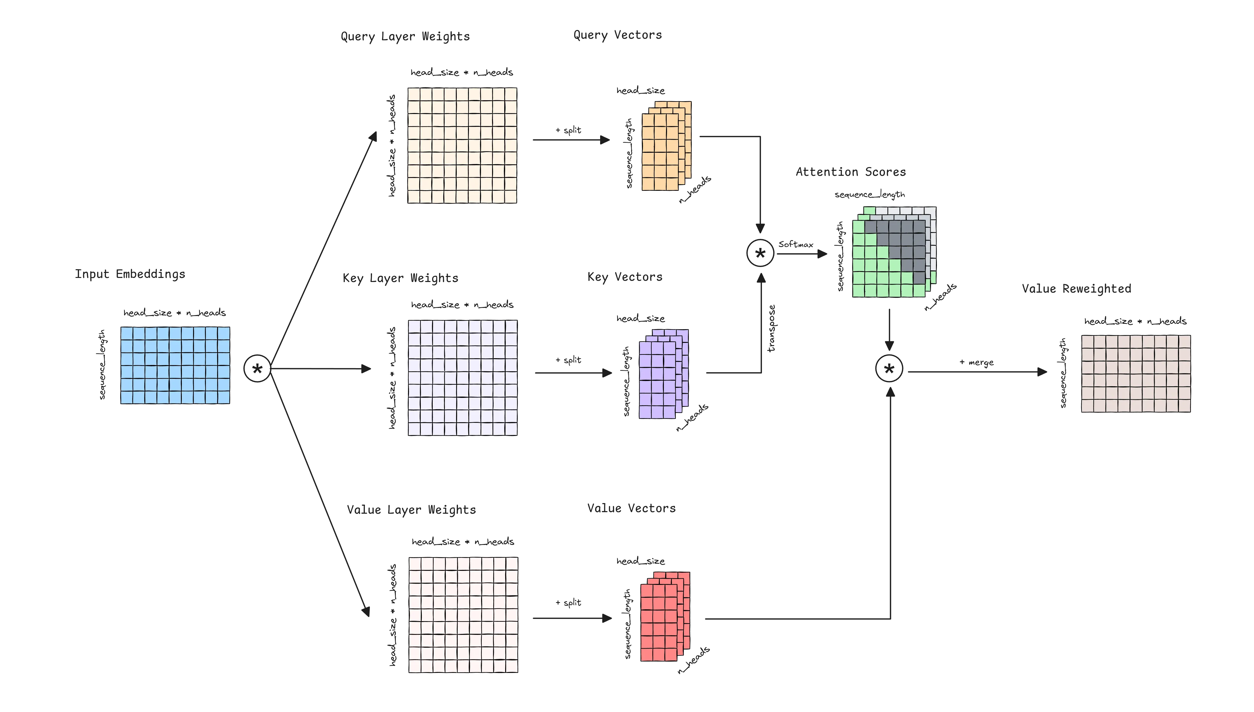
In code, the three projections keep the same number of heads, and the heads are just a reshape of the projected vectors:
class MultiHeadAttention(nn.Module):
    def __init__(self, n_embd, n_heads):
        super().__init__()
        self.n_heads = n_heads
        self.head_size = n_embd // n_heads

        self.q_proj = nn.Linear(n_embd, n_heads * self.head_size, bias=False)
        self.k_proj = nn.Linear(n_embd, n_heads * self.head_size, bias=False)
        self.v_proj = nn.Linear(n_embd, n_heads * self.head_size, bias=False)
        self.out_proj = nn.Linear(n_embd, n_embd, bias=False)

    def forward(self, x):  # x: (batch, seq, n_embd)
        batch, seq, _ = x.shape

        q = self.q_proj(x).view(batch, seq, self.n_heads, self.head_size)
        k = self.k_proj(x).view(batch, seq, self.n_heads, self.head_size)
        v = self.v_proj(x).view(batch, seq, self.n_heads, self.head_size)
        # (batch, seq, n_heads, head_size) -> (batch, n_heads, seq, head_size)
        q, k, v = (t.transpose(1, 2) for t in (q, k, v))

        # attention scores: (batch, n_heads, seq, seq)
        att = (q @ k.transpose(-2, -1)) / math.sqrt(self.head_size)
        causal = torch.ones(seq, seq, dtype=torch.bool, device=x.device).tril()
        att = F.softmax(att.masked_fill(~causal, float("-inf")), dim=-1)

        out = att @ v  # (batch, n_heads, seq, head_size)
        out = out.transpose(1, 2).reshape(batch, seq, -1)  # concatenate the heads
        return self.out_proj(out)
KV-Cache
Transformer models are huge and different optimization techniques appeared to speed up the inference. The objective of our model inference is to produce the next token that follows the last token in the intput sequence (next token prediction). What do we need to compute this? Just the final embedding of the last token , the last token representation of the Value Reweighted.
To obtain this embedding, last token representation of the Value Reweighted, we need to compute the dot product between the Attention Scores and the Value Vectors.
The Value Layer Weights are allways the same, as we are at inference, then Value Vectors for the tokens previous to the last token are the same and we just need to compute the new last one. We can cache Value Vectors from previous tokens and reuse them .
Regarding the Attention Scores , for obtaining the last token representation of the Value Reweighted we just need the Attention Scores of the last token. For calculating this final attention row, we just need the Query Vectors of the last token and make the dot product with all the Key Vectors. But the Key Vectors from previous tokens are the same than when were computed in the previous step, then we can cache Key Vectors from pevious tokens and reuse them .
And with this last token embedding and the Key and Value vectors cached, we can iterate over the Transformer blocks and compute the final embedding of the last token representation.
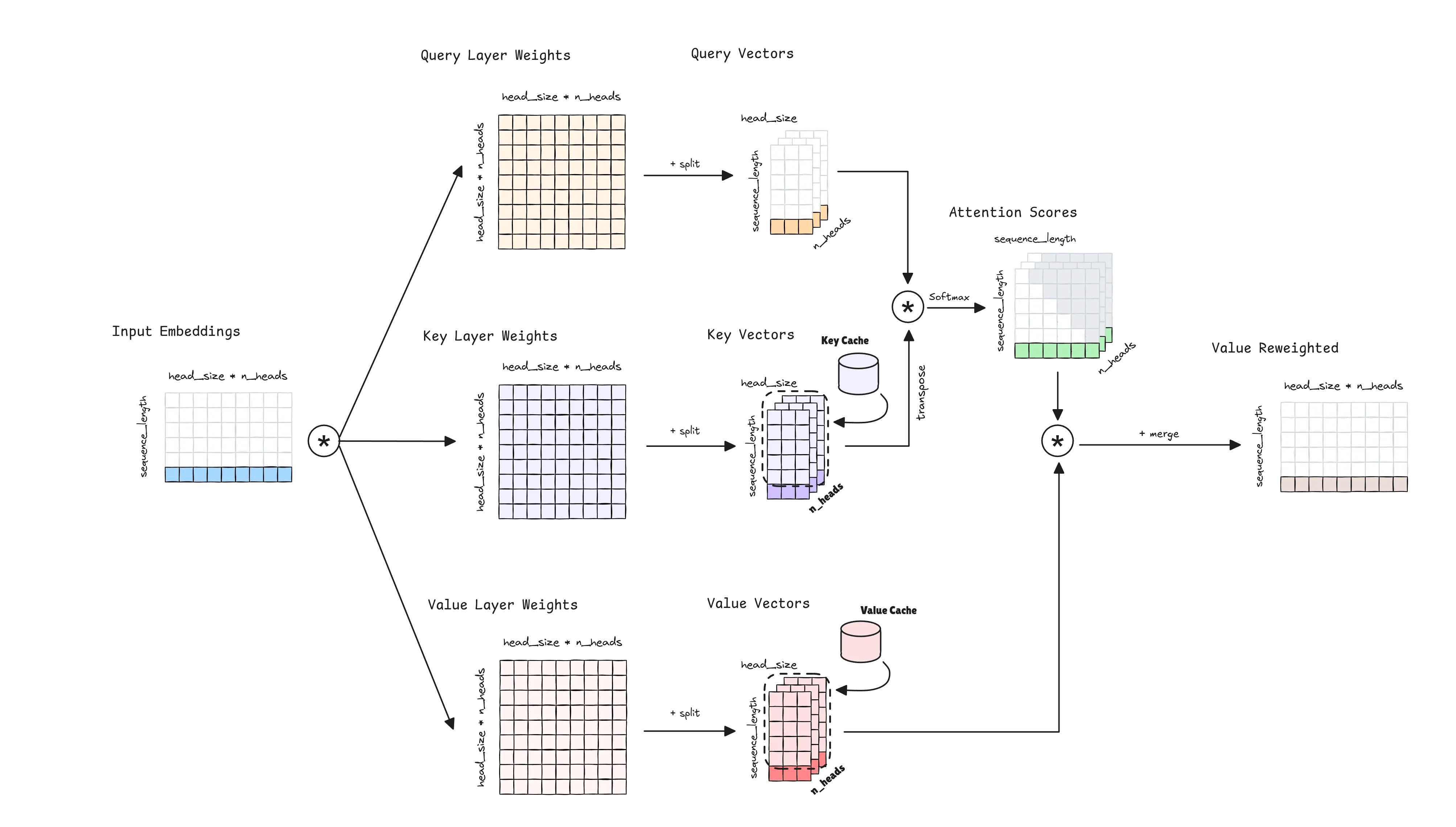
¿Why don’t we cache the Query Vectors? Because we don’t need all the Query Vectors, just the last one. For calculating the last token Value Reweighted we just need the Attention Scores of the last token, and for that one we just need the last Query Vector.
The implementation barely changes: the layer receives only the new tokens, concatenates their Key and Value vectors to the cached ones, and returns the updated cache.
class MultiHeadAttention(nn.Module):
    # ...

    def forward(self, x, cache=None):
        # x holds only the new tokens: while decoding, seq == 1
        batch, seq, _ = x.shape
        # ... same projections as before, each (batch, n_heads, seq, head_size)

        if cache is not None:
            past_k, past_v = cache
            # (batch, n_heads, past + seq, head_size)
            k = torch.cat([past_k, k], dim=2)
            v = torch.cat([past_v, v], dim=2)

        att = (q @ k.transpose(-2, -1)) / math.sqrt(self.head_size)
        if seq > 1:  # only the first pass, over the prompt, has a future to hide
            causal = torch.ones(seq, seq, dtype=torch.bool, device=x.device).tril()
            att = att.masked_fill(~causal, float("-inf"))
        att = F.softmax(att, dim=-1)

        out = (att @ v).transpose(1, 2).reshape(batch, seq, -1)
        return self.out_proj(out), (k, v)
Note that the causal mask is only needed for the first pass: when decoding, the single query is the last token, so it is entitled to attend to every cached key.
Generation then splits in two phases, prefill , where the prompt goes through the model once and fills the cache, and decode , where each step only projects the token just generated:
@torch.no_grad()
def generate(model, prompt, max_new_tokens):
    logits, cache = model(prompt)  # prefill: (batch, prompt_len) -> cache

    tokens = []
    for _ in range(max_new_tokens):
        next_token = logits[:, -1:].argmax(-1)  # (batch, 1)
        tokens.append(next_token)
        # decode: one token in, the whole context read from the cache
        logits, cache = model(next_token, cache)

    return torch.cat(tokens, dim=1)
In a real model the cache is not a single pair but one pair of Key and Value tensors per layer.
Without it, every step would re-project and re-attend over the entire prefix,
turning the generation of tokens into work per layer instead of .
Caching the Key and Value Vectors, we can save computations and speed up the inference process. The cost of caching those vectors is , where the final terms correspond to the number of caches per layer (one for Key and one for Value), and the number of bytes per floating point value (assuming each model parameter is a 16-bit floating point value), respectively. The rest of the terms are:
| Hyperparameter | Description |
|---|---|
| Number of Transformer layers in the model. | |
| Batch size. | |
| Number of attention heads. | |
| Head hidden size. | |
| Sequence length. |
Can we further reduce the cache needed? Yes, we can! By reducing the size of the cache, improving the load and therefore the speed of inference and also the memory required. That is, at the cost of some of the performance of our model.
Multi-Query Attention
If we look closer at the Multi-Head Attention mechanism, we can see that the Key and Value Vectors have different set of weights for each head. How can we reduce the cache needed for the Key and Value Vectors? Simple, we can reduce the number of Key and Value heads needed. Particularly, Multi-Query Attention proposes to use a single set of Key and Value Vectors. This obviously will reduce the capacity of the model to capture different aspects of the relationships between tokens, we have less heads to model the relationships, and therefore the performance of the model will be affected. But, it will reduce the cache needed and the inference time.
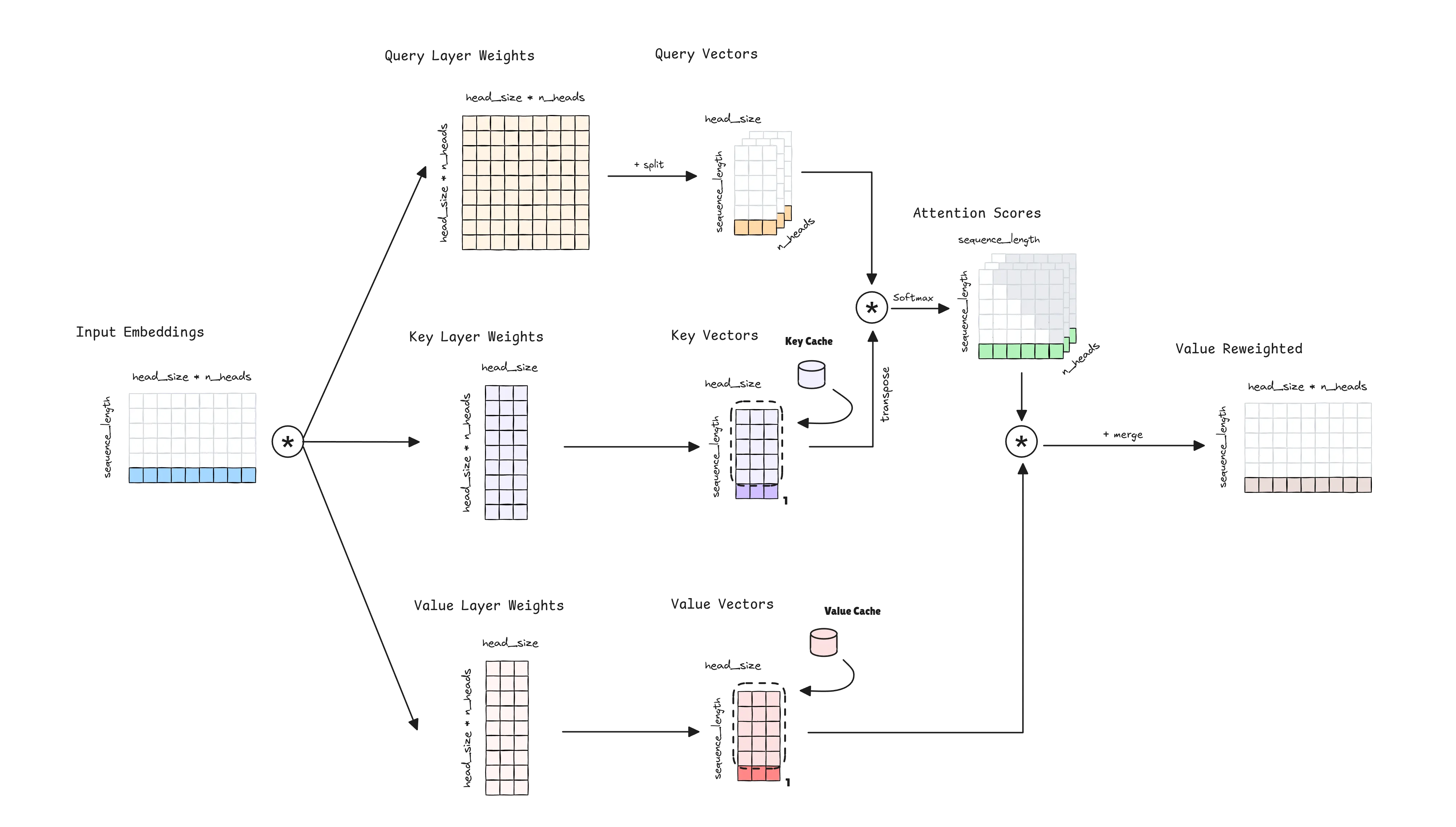
The cost of caching the Key and Value Vectors is . Note how the number of attention heads is not present in the formula.
The only structural change is in the Key and Value projections, which now output a single head:
class MultiQueryAttention(nn.Module):
    def __init__(self, n_embd, n_heads):
        super().__init__()
        self.n_heads = n_heads
        self.head_size = n_embd // n_heads

        self.q_proj = nn.Linear(n_embd, n_heads * self.head_size, bias=False)
        # a single Key/Value head, shared by every query head
        self.k_proj = nn.Linear(n_embd, self.head_size, bias=False)
        self.v_proj = nn.Linear(n_embd, self.head_size, bias=False)
        self.out_proj = nn.Linear(n_embd, n_embd, bias=False)

    def forward(self, x, cache=None):
        batch, seq, _ = x.shape

        q = self.q_proj(x).view(batch, seq, self.n_heads, self.head_size)
        q = q.transpose(1, 2)            # (batch, n_heads, seq, head_size)
        k = self.k_proj(x).unsqueeze(1)  # (batch, 1, seq, head_size)
        v = self.v_proj(x).unsqueeze(1)

        # ... cache concatenation and masking, identical to before
        att = (q @ k.transpose(-2, -1)) / math.sqrt(self.head_size)
        out = att @ v  # (batch, n_heads, seq, head_size)

        out = out.transpose(1, 2).reshape(batch, seq, -1)
        return self.out_proj(out), (k, v)
The head dimension of the Key and Value vectors is now , so it is broadcast against the query heads: no copy is materialized, and the cache stores one head instead of .
Inefficient Parallelization
Many large Transformer models require more memory than can fit on a single GPU, employing model parallelism to distribute the model across multiple GPUs. This is accomplished usually with Tensor Parallelism, assigning different attention heads to different GPUs.
For example, 175B GPT-3 model has 96 attention heads, and if we have 8 GPUs, we can assign 12 heads to each GPU.
Each GPU performs the entire attention computation for its assigned heads, then all GPUs exchange the results of their computations. With Multi-Query Attention, each attention head has the same set of Key and Value Vectors, computing and caching the same set of Key and Value Vectors in each GPU. This is inefficient, as we are computing the same values in each GPU at the same time we are reducing the capacity of the model.
Grouped-Query Attention
Grouped-Query Attention tries to solve the inefficient parallelization of Multi-Query Attention. To do so, it proposes to increase the number of Key and Value Vectors heads to an arbitrary number, an hyperparameter . The Query Vectors are grouped in groups, and each group has a different set of Key and Value Vectors.
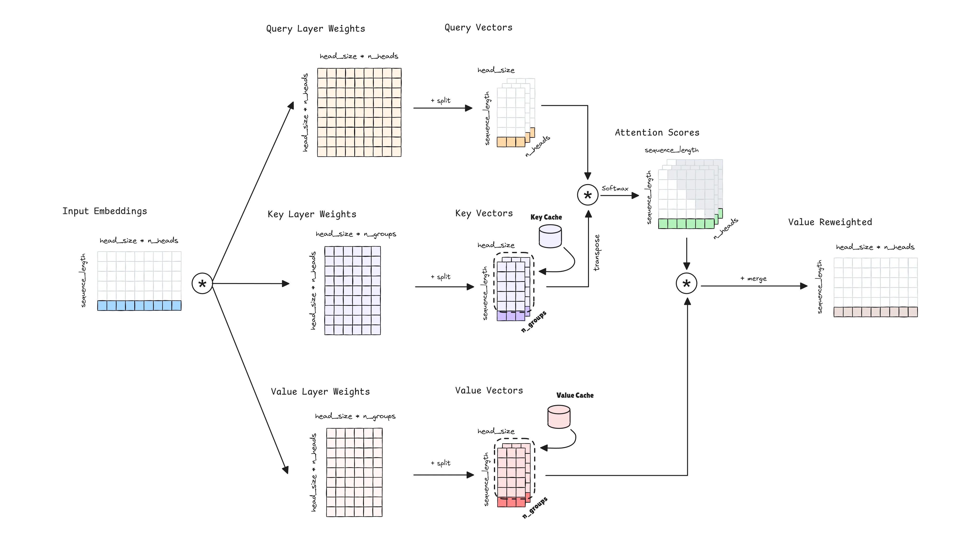
When operating in a multi-GPU environment with tensor parallelism, we can essentially get the same speed up as Multi-Query Attention by setting equal to the number of GPUs, but with the advantage of providing the model with more capacity and performance. The cost of caching the Key and Value Vectors is . Note how the number of attention heads is not present in the formula, being replaced by the hyperparameter .
In code, becomes the n_kv_heads hyperparameter, and each Key/Value head
is shared by a group of n_heads // n_kv_heads query heads:
class GroupedQueryAttention(nn.Module):
    def __init__(self, n_embd, n_heads, n_kv_heads):
        super().__init__()
        assert n_heads % n_kv_heads == 0
        self.n_heads, self.n_kv_heads = n_heads, n_kv_heads
        self.group_size = n_heads // n_kv_heads  # query heads per Key/Value head
        self.head_size = n_embd // n_heads

        self.q_proj = nn.Linear(n_embd, n_heads * self.head_size, bias=False)
        self.k_proj = nn.Linear(n_embd, n_kv_heads * self.head_size, bias=False)
        self.v_proj = nn.Linear(n_embd, n_kv_heads * self.head_size, bias=False)
        self.out_proj = nn.Linear(n_embd, n_embd, bias=False)

    def forward(self, x, cache=None):
        batch, seq, _ = x.shape

        q = self.q_proj(x).view(batch, seq, self.n_heads, self.head_size)
        k = self.k_proj(x).view(batch, seq, self.n_kv_heads, self.head_size)
        v = self.v_proj(x).view(batch, seq, self.n_kv_heads, self.head_size)
        q, k, v = (t.transpose(1, 2) for t in (q, k, v))

        if cache is not None:
            past_k, past_v = cache
            k = torch.cat([past_k, k], dim=2)
            v = torch.cat([past_v, v], dim=2)
        new_cache = (k, v)  # cached before repeating: only n_kv_heads are stored

        # each Key/Value head serves its group of query heads
        k = k.repeat_interleave(self.group_size, dim=1)
        v = v.repeat_interleave(self.group_size, dim=1)

        # ... attention and masking, exactly as in Multi-Head Attention
        return self.out_proj(out), new_cache
Two details worth keeping in mind. The cache is filled
before repeating the heads , otherwise we would be storing the
copies we were trying to avoid. And repeat_interleave is written here for clarity,
while optimized kernels read the shared heads directly, without materializing the copies.
Note that this single implementation covers the three mechanisms:
n_kv_heads = n_heads is Multi-Head Attention, n_kv_heads = 1 is Multi-Query Attention,
and anything in between is Grouped-Query Attention.
Speed ups references
To put in context the speed ups of the different attention mechanisms, we can see the following table:
| Model | Parameter Count | KV Cache Size MHA | KV Cache Size MQA | KV Cache Size MGA |
|---|---|---|---|---|
| GPT-3 | 175B | 4.5GB | 48MB | 384MB |