Depthwise Separable Convolutions

Commonly used in networks as MobileNet, the depthwise separable convolutions consists of two steps: depthwise convolutions and $1\times1$ convolutions.

Standard convolution

Before describing the depthwise separable convolution, it is worth revisiting the typical convolution. For a concrete example, let’s say an input layer of size $7\times7\times3$ (height $\times$ width $\times$ channels), and 128 filters of size $3\times3\times3$, after applying one filter, the output layer is of size $5\times5\times1$ (only 1 channel), and grouped up with the 128 filters, $5\times5\times128$.

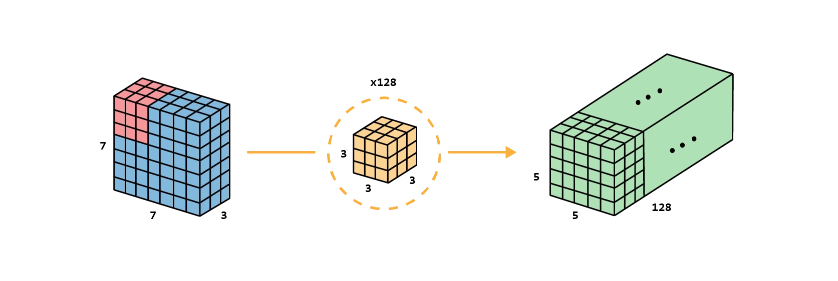
Illustrated through code:

# Input volume with depth 3 and outputs 128 kernels
# Uses 3×3 convolutional kernel
conv_layer = nn.Conv2d(in_channels=3, out_channels=128, kernel_size=3)

Depthwise Separable Convolutions

Let’s see how we can achieve the same transformation as the standard convolution with less computation .

We first apply depthwise convolution to the input layer. Instead of using a single filter of size $3\times3\times3$, we will use 3 kernels separately . Each filter has a size of $3\times3\times1$, each kernel convolves with 1 channel of the input layer ( 1 channel only, not all channels! ). Each such convolution, in the example, will provide a map of size $5\times5\times1$, and we will stack them to create a $5\times5\times3$ image. We shrunk the spatial dimension, but the depth is still the same as before.

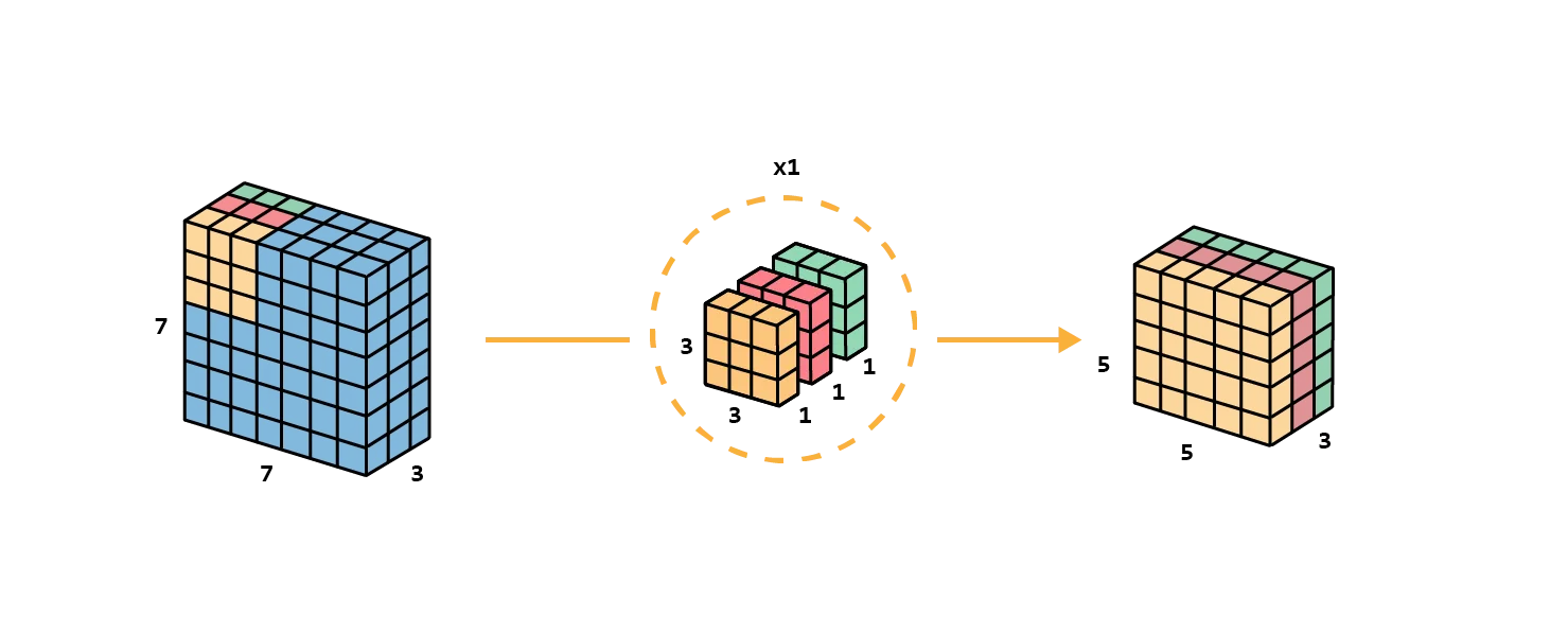
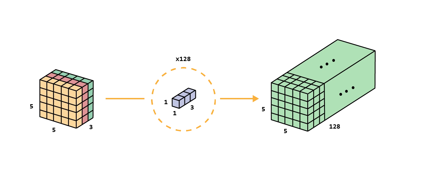
Then, it’s time for the second step, extend the depth by applying $1\times1$ convolutions , as many as the depth we want to achieve, as for the example 128 filters.

With these steps, we also (as in the standard convolution) transform the input layer $7\times7\times3$ into the output layer $5\times5\times128$ as for the standard convolution. The overall process of the depthwise separable convolution would be:

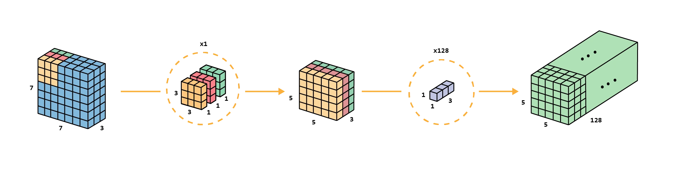
Which would be defined as:

# Define depthwise separable convolutional layer
# Note how we use the groups parameter: At groups equals to in_channels,
# each input channel is convolved with its own set of filters
depthwise_conv_layer = nn.Conv2d(
	in_channels=3, out_channels=3, kernel_size=3, groups=3
)
pointwise_conv_layer = nn.Conv2d(
	in_channels=3, out_channels=128, kernel_size=1
)

The advantage of doing depthwise separable convolutions is the efficiency . One needs much less operations for depthwise separable convolutions compared to standard convolutions.

Meanwhile for the standard convolutions we need to move 128 filters with dimensionality $3\times3\times3$ around the input $5\times5$ times, i.e., $128\times3\times3\times5\times5 =$ 86400 multiplications, the depthwise separable convolution uses 3 kernels $3\times3\times1$ that moves $5\times5$ times, and after that, 128 filters of dimensionality $1\times1\times3$ that moves $5\times5$ times over the previous output, i.e., $3\times3\times3\times1\times5\times5 + 128\times1\times1\times3\times5\times5 =$ 9600 multiplications, only about the 12% of the cost of the standard convolution (for this example convolution configuration).

References

• A Comprehensive Introduction to Different Types of Convolutions in Deep Learning
• Designing Faster Neural Networks