The Receptive Field in Convolutional Neural Networks

Why do architectures use $3\times3$ filters? It is because of something called Receptive Fields. In this post, we will see what is the receptive field and how it increases over convolutional layers. Taking this into account, we will see why architectures use $3\times3$ filters.

What is the Receptive Field?

The receptive field is the area of the input image that affects a particular unit of the network. In other words, it is the area of the input image that contributes to the calculation of a particular unit in the network.

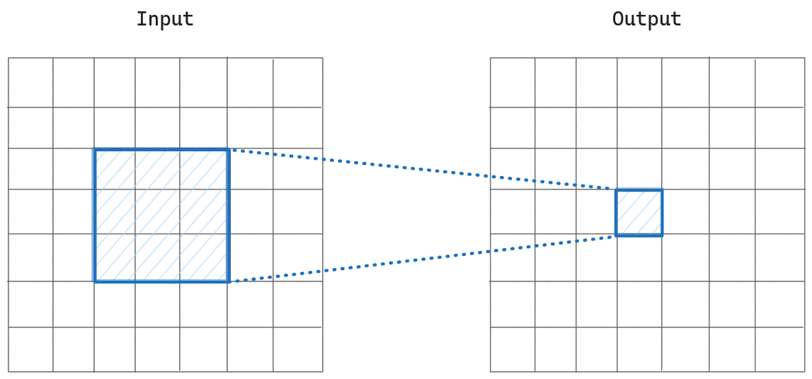
Single Kernel Case

We have our input image and we pass it through $3\times3$ convolution layers until we get the output. If we pick an output pixel from the output, that pixel depends on the $3\times3$ receptive field of the previous feature map, so we can say that the receptive field size of the pixel of the output is 3 so far.

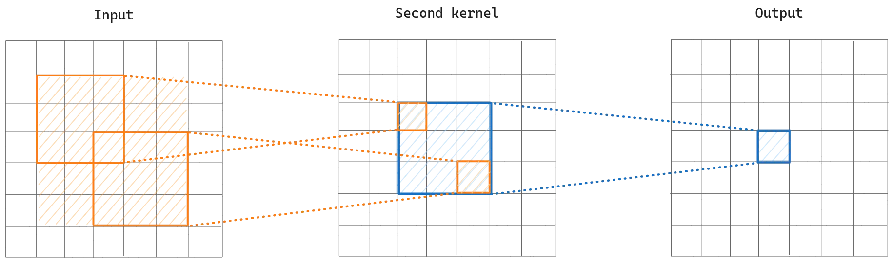
Multiple Kernels Case

Let’s see what happens to receptive field size after adding the second layer to our calculation. We see that if we pick the corner pixels that are involved in the initial receptive field, those provide from a larger $5\times5$ receptive field. If we recap, till now we have a pixel on the output that it depends on $3\times3$ receptive field of its previous layer, which depends on the $5\times5$ receptive field of the second layer. In other words, if we put two $3\times3$ convolution layers subsequently it has the effect of putting one $5\times5$ convolution layer.

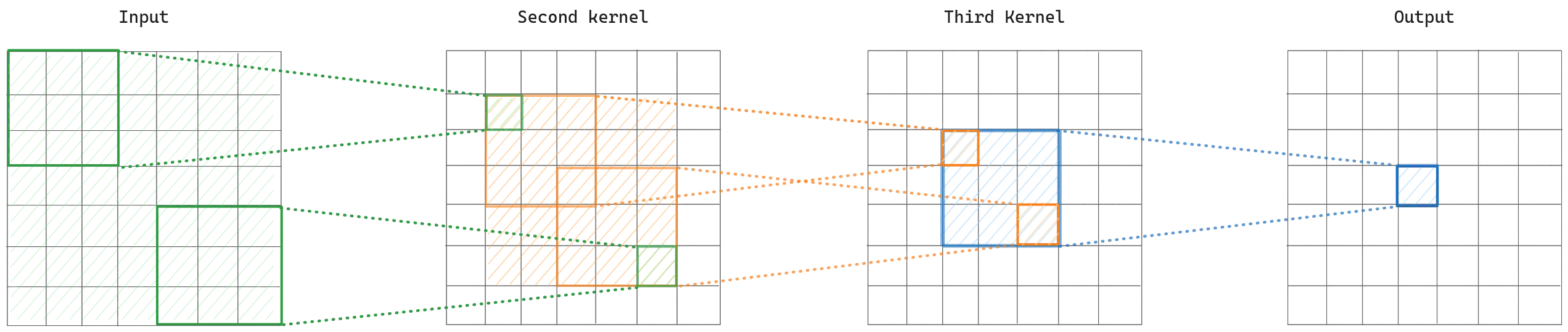
Now let’s add a third layer to our calculation. Again we select the corner pixels and then find the receptive field of them in the input layer. We can see that it covers the $7\times7$ area, which is the whole input. In other words, every pixel in the output feature map contains information of the whole input image, and generally, as we go further, we have higher semantic information.

If we formulate how receptive field increases as we add more convolutional layers. The first convolution adds to our receptive field size the same as the kernel size. The next one adds two, and the final one adds two too. If we generalize this, we can say the first convolution adds the $kernel\ size$ and previous ones add $kernel\ size - 1$. Assuming having $L$ layers, the receptive field size is $k+(L-1)(k-1)$ which is the same as $1 + L(k-1)$.

To better understand how receptive field size increases over convolutional layers, I recommend to read the application of the convolution operations backwards, from the output to the input.

Why do architectures use 3x3 filters?

What is the problem with $5\times5$ or $7\times7$ convolutions? Imagine we have an input volume having $C_1$ channels.

In the first scenario we use $5\times5$ kernels which of course should have the same number of channels $C_1$ as the input volume and a number of kernels $C_2$. The number of parameters is $(5\times5)C_1 C_2 = 25C_1 C_2$.

In another scenario, we have another input volume with the same number of channels $C_1$, we will have $C_2$ kernels as output, but this time we will use two 3×3 kernels subsequently instead, as we know a 5×5 kernel has the same receptive field as two 3×3. The number of parameters is $(3\times3)C_1 C_2 + (3\times3)C_1 C_2 = 18C_1 C_2$.

We can see that the number of parameters, as for the number of operations, is lower by using two $3\times3$ kernels subsequently. A final advantage of using two $3\times3$ kernels subsequently instead a $5\times5$ kernel is that when using $3\times3$ kernels when introduce in between activation maps which adds more non-linearity to our model.

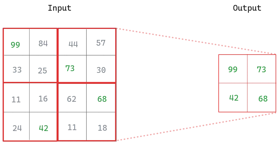
The Pooling layers

Imagine we have an input size of $224\times224$ and our kernel size is $3$. Based on the formula that receptive field is $1 + L(k-1)$ we can write $1+L(3-1) =224 \rightarrow L \approx 112$. That basically means that we need to add $112$ $3\times3$ convolution layers to our neural network so at the end every pixel could capture the whole information that exists in the image. That’s the reason we use pooling layers.

If we apply a Max Pooling with kernel size $2\times2$ and stride 2, for every two rows and every two columns we only have one single value. So that max pooling always doubles the size of our receptive field size, for that kernel and stride configuration, which basically means that we don’t need to have a very deep neural network.

Credits

• Receptive Fields: Why 3x3 conv layer is the best?
• Designing Faster Neural Networks
• Receptive Fields CNN Excalidraw diagram source